We learn most things in life by making mistakes, getting feedback (success/failure), and then trying again and again until we reach our goal. Well, Reinforcement Learning (RL) brings this human learning process into computers, by letting them learn and improve on their own, just like us!
What is RL?
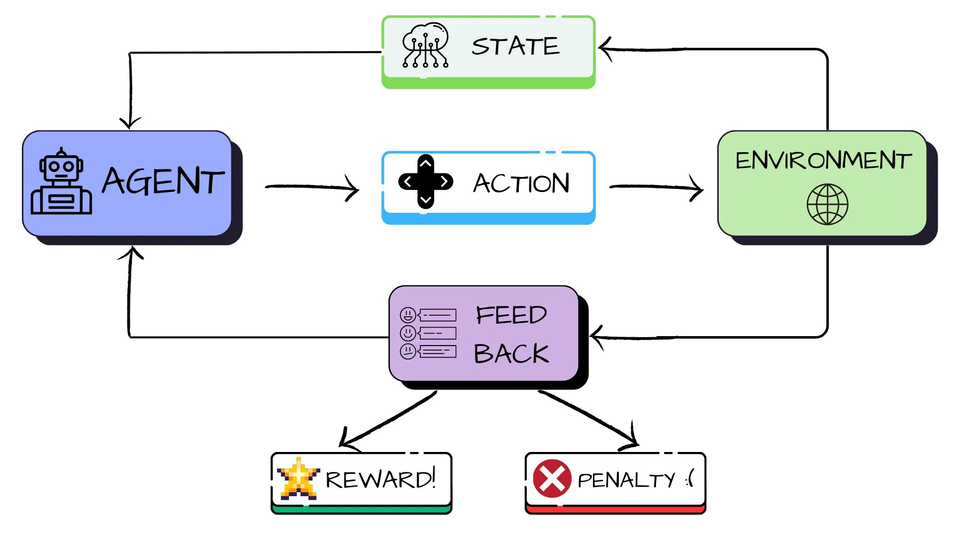
Reinforcement learning is a way for machines to learn by taking ‘actions’ in a particular ‘state’ of an ‘environment’, making ‘observations’, and gradually performing better actions through ‘feedback’.
Instead of being told what the right answer is, they discover strategies for success by trial-and-error.
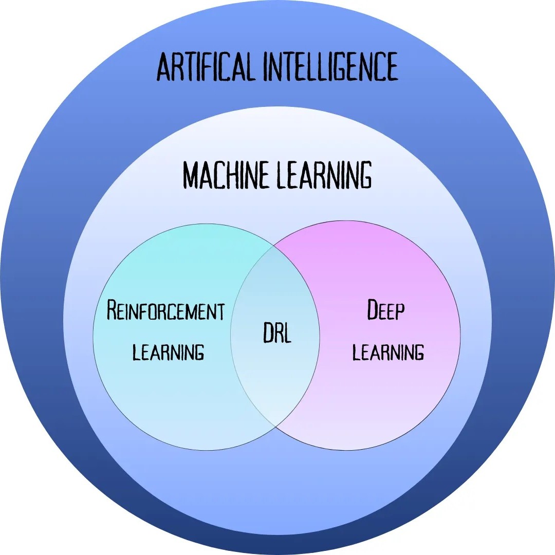
As we know, ML is a core subset of AI. Within that comes:
- Reinforcement Learning — strategy for learning through trial and error
- Deep Learning — powerful computer brain, called a neural network
When you put these together, you get Deep Reinforcement Learning (DRL), where a neural network learns using the trial-and-error process.
RL is mainly used where the problem cannot be solved by looking up answers in a fixed dataset, but the agent can interact with an environment and create its own data.
For example: A city for self-driving cars.
No matter how many rules you feed a machine, you can’t predict every scenario. So, the main goal here is to minimize errors, not predict every move.
Keywords and Processes
Let’s understand RL better by taking an everyday example.
You are a student and you’re starving after back-to-back lectures, and the only way to get food on campus is the canteen.
The problem is, it’s always packed, and if you want a seat, you will have to wait at least 10 mins and then be ready to sprint as soon as someone stands up. Each time you try, you note three things.
- How long you waited
- How good the food was
- How much time you have left before your next class
Over time, you try different strategies to know how you can get food quickly and still make it to class on time.
Now, using the definition I mentioned earlier, let’s identify what each RL keyword means w.r.t. our canteen example.
- Agent: the one who perform actions (you!)
- Environment: the “world” in which the agent behaves and makes choices. (crowded canteen)
- State: this is the current situation that describes where exactly the agent is inside the environment. (how hungry, time to next class, crowd level)
- Action: its the decision that the agent makes. (scan for empty tables, wait nearby)
- Feedback: the response the agent gets after taking an action. It’s positive (reward) for reaching the goal or negative (punishment) for failing to reach the goal. The reward varies on how fast the goal was achieved. The lesser time taken, the higher the reward is and vice versa. (food and class on time = reward, missing food = punishment)
- Policy: Agent’s overall strategy/rules developed over time
Repeat. The agent repeats this entire process, and learns from each round and improves its policy. So, in our example, you use your past experiences to try new ways to get a seat and the food faster.
Once our agent knows how to reach the target — getting a seat and food in this case, it has two options for future actions:
-
Exploitation: Now that the agent knows how to reach the target, it always does that action since it thinks that’s what will give the highest reward (based on its experience so far). Here, it will be you always going to the table that got you food fastest last week.
-
Exploration: Trying new actions, even if its not sure that it will be the best. This is so that you can discover better rewards later. Here, you waiting by a different table today to see if it gets you food faster is exploration.
RL agents usually start with higher exploration rates, trying every option to learn what works best. Gradually, as they get smarter, this exploration rate is tuned down and they focus on exploiting the best moves that they found.
The Blueprint: Markov Decision Process (MDP)
Markov process depends on the “Markov property,” which models situations such that the next step depends only on the current step and not on how you got there.
“Future depends only on the present, not the past.”
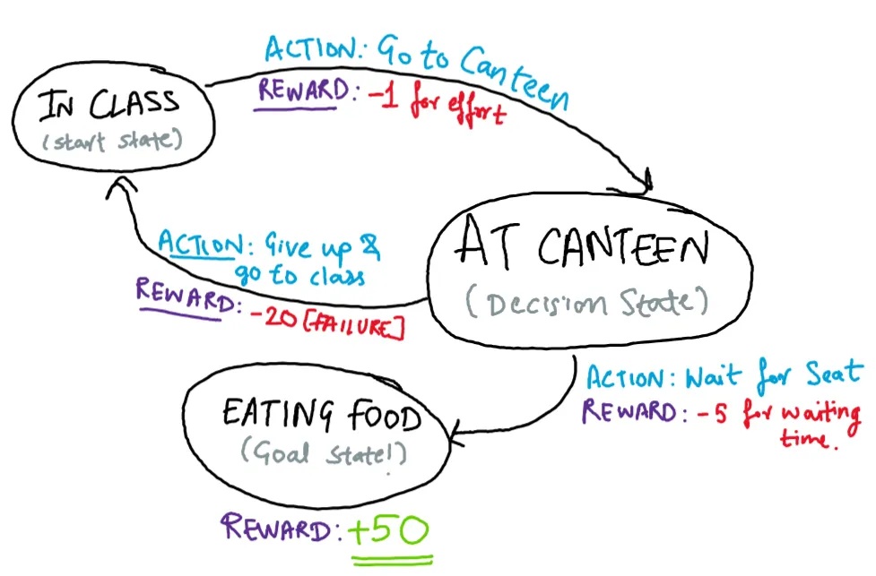
MDP is the ‘blueprint’ for our RL agent. It doesn’t solve the problem, but gives it a structure by defining all possible states, available actions, and rules for rewards. Our agent’s job is to use this blueprint to find the best possible path to reach the target (optimal policy).
Comparing ML Types: Supervised, Unsupervised, and RL
Now that we know what RL is, let’s see how it stands apart from other machine learning types like supervised and unsupervised learning.
| Supervised | Unsupervised | RL | |
|---|---|---|---|
| Data Input | The data is labelled, i.e., the answers are provided beforehand | Unlabeled data. No answers are given. | Raw experience, it learns from the environment |
| Learning Style | Learns from examples with answers | Spots patterns or groups in data | Learns by interacting and getting feedback |
| Goal | Get as many correct answers as possible | Find hidden patterns or groupings in the data | Learn a policy to maximise long-term reward |
| Feedback Type | Immediate and direct (correct/incorrect) | No feedback during training | Indirect or delayed (only after seeing the result of the action) |
| Example | Show the computer apple images and label them “apple”. It learns to identify apples from these labeled examples. | Give the computer lots of fruit images without labels. It finds out on its own which look similar, grouping apples together. | The computer guesses if an image is an apple and only learns from your reward or punishment after each guess, and improves over time. |
Types of RL Algorithms
Before learning the algorithms, it’s really important that we learn what Q-function is first, in context of all the terminologies we have learnt so far.
To know that, let’s see how to calculate ‘Rt’ which is the discounted sum of all the individual rewards ( r ) over time ( t ).
‘γ’ (gamma) here lies between [0, 1] and represents the discount factor (patience level).
If its low (eg: 0.1) that means our agent is impulsive. It’s like saying “I would rather have 10 bucks now instead of 100 rupees in the future”.
If its higher (eg: 0.99), it means our agent is patient and says “I’ll have 100 bucks in the future because its a higher reward”.
So, what exactly does Q-function do?
It captures the “expected” total future reward an agent in state “s” can receive by performing an action “a”.
Now that we understand what the Q-function represents, let’s see how reinforcement learning algorithms use these ideas in practice through two fundamental approaches:
Value Learning
The main goal here is to figure out how “good” or “valuable” each situation is.
-
Find Q(s, a): You first learn the Q-function, that calculates a “score” or “Q-value” for every possible action (a) in every state (s).
-
Find a:
This says “Action (a) that I chose is the one that gives the maximum possible Q-value w.r.t my current state.” The agent calculates the score for all actions and greedily picks the best one.
In summary, it rates every action which is possible for a given state and then picks the one which has the highest rating.
Policy Learning
This strategy does not assign a score, but instead learns a policy π(s) which is a set of rules for what to do in a given situation (state)
- Find π(a|s):
This formula tells us the probability that our agent will take a specific action () given that it is in a specific state (), under the policy π at time t.
- Sample a ∼ π(s): This means, “I will sample my next ‘a’ based on the strategy given by my policy (π) for the current ‘s’.” The policy might give a probability for each action (e.g., “70% chance you should go left, 30% chance you should go right”).
Simply put, the agent is like a chess player who has memorized a guidebook. It doesn’t score every possible move but it just knows the best move to make in a given situation based on the strategy given in that guidebook.
Q-leaning and DQN
Q-learning (The foundation)
It is the ‘foundational’ algorithm (Watkins, 1989) for learning a value function. The main goal is to learn the “quality” (Q-value) of every possible action in every possible state.
- It is a type of value learning algorithm. Q-Learning stores these Q-values in a simple spreadsheet-like structure called a “Q-Table”.
It has a row for every possible state and a column for every possible action. Each cell in the table holds a numerical score (Q-value) for that specific state-action pair. Higher the Q-value, higher is the satisfaction rate.
Circling back to our canteen example, its q-table will look something like this:
| State (Current Situation) | Action: “Wait by Kitchen” | Action: “Scan for Tables” | Action: “Wait by Door” |
|---|---|---|---|
| Canteen is Crowded | 8.5 | 6.2 | 3.1 |
| Canteen is Moderate | 7.0 | 7.8 | 5.5 |
| Canteen is Empty | 2.0 | 5.0 | 9.0 |
The agent constantly updates the scores in this Q-table (while exploring) using the Bellman Equation:
Where:
Q_new (s,a)- new score for our action.Q_old (s,a)- old score we are updating.α- Learning Rate (usually a small number).R(s,a)- immediate reward we just got.γ- discount factor- - best possible score we could get from the next state we landed in.
DQN (The POWERFUL Upgrade)
To handle worlds with millions of states, we replace the Q-table with a deep neural network. This combination is called a Deep Q-Network (DQN).
We can use deep neural networks in place of q-tables in the following ways:
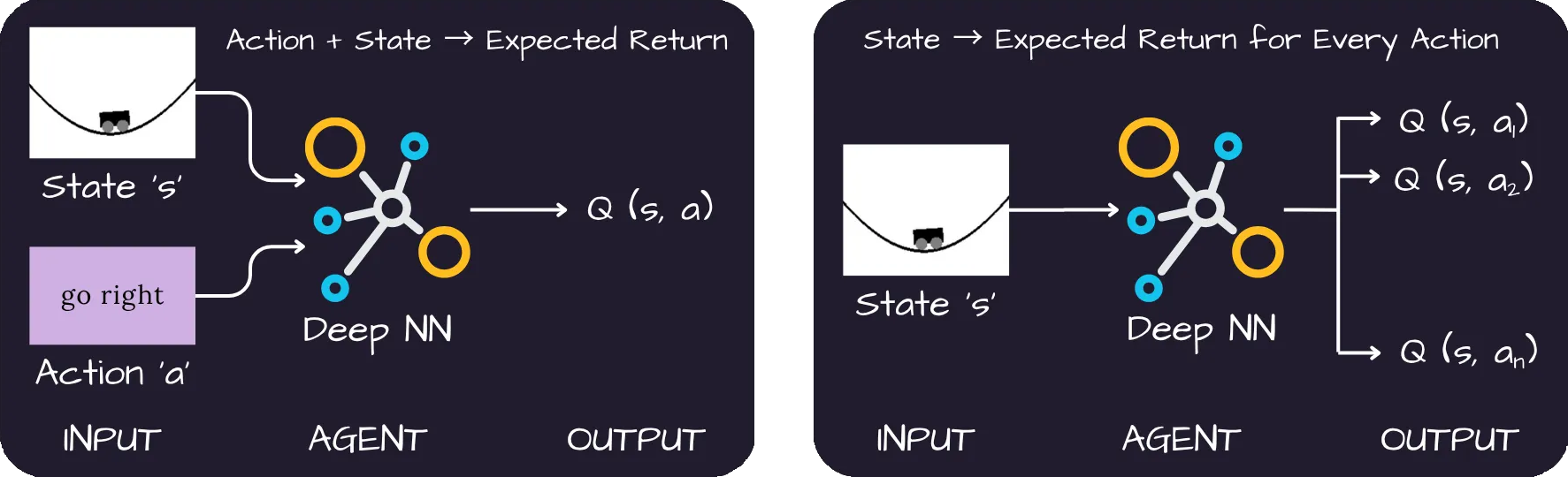
Experience Replay — a DQN agent stores its experiences (state, action, reward, next_state) in a “memory bank.” It then learns by replaying random samples of these past experiences, which makes the training process much more stable and efficient than a simple Q-table.
DQN working:
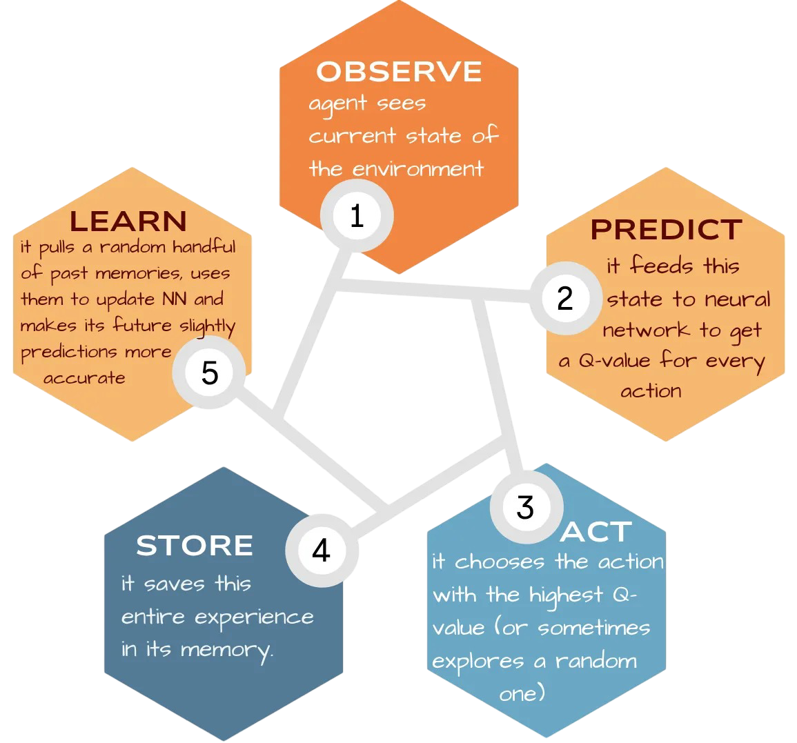
This helps the DQN to master complex tasks, from classic control problems to video games.
Implementing MountainCar with DQN
To see DQN in action, I decided to solve the classic Reinforcement Learning challenge: MountainCar.
- MountainCar is a built-in setup from Python’s gymnasium library.
The problem at hand is, our agent’s (the car) accelerator isn’t strong enough to drive uphill to reach the target. So, our agent needs to learn to take a negative action (going left, i.e. away from target) to gain momentum and then accelerating in the right direction to reach the target.
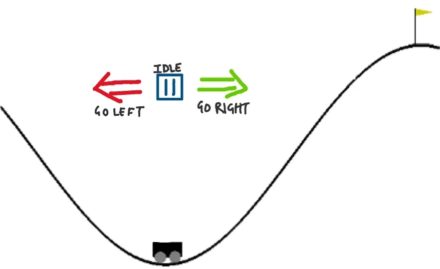
| The Agent 🤖 | DQN algorithm (“brain” that learns the driving strategy) |
|---|---|
| Environment 🏞️ | MountainCar world (gymnasium library) |
| State 📊 | [car_position, car_velocity] |
| Actions 🕹️ | 1. Go left (0) 2. Do nothing (1) 3. Go Right (2) |
| Reward 🏆 | -1 penalty for every time step the car has not reached the flag. (A large positive reward is given only when the car successfully reaches the goal.) |
Let’s start by importing the necessary libraries
# imports and environment setups
import gymnasium                # RL environments
import numpy as np              # numbers and arrays
import torch                    # PyTorch (tensors + training)
import torch.nn as nn           # neural network layers
import torch.optim as optim     # optimizers like Adam
from collections import deque   # fast queue for replay buffer
import random                   # random choices
import matplotlib.pyplot as plt # plotting
Now we will define our q-network
# defining our Q-network: a small 3-layer neural network
class QNetwork(nn.Module):
    def __init__(self, state_size, action_size):
        super(QNetwork, self).__init__()
        # blueprint (layers): input -> hidden -> hidden -> output
        self.fc1 = nn.Linear(state_size, 64)  # takes the game state
        self.fc2 = nn.Linear(64, 64)          # processes information
        self.fc3 = nn.Linear(64, action_size) # outputs a score (Q-value) per action

    def forward(self, x):
        # the flow: pass state through layers with ReLU, then get Q-values
        x = torch.relu(self.fc1(x))
        x = torch.relu(self.fc2(x))
        return self.fc3(x)  # final Q-values for each action
Let’s create a Memory Bank for Our Agent (Experience Replay)
# replay buffer: stores and samples experiences for training
class ReplayBuffer:
    def __init__(self, capacity):
        self.buffer = deque(maxlen=capacity)

    def push(self, state, action, reward, next_state, done):
        # save one experience tuple
        self.buffer.append((state, action, reward, next_state, done))

    def sample(self, batch_size):
        # pick a random mini-batch
        batch = random.sample(self.buffer, batch_size)
        states, actions, rewards, next_states, dones = zip(*batch)
        return (np.array(states), np.array(actions), np.array(rewards),
                np.array(next_states), np.array(dones))

    def __len__(self):
return len(self.buffer)- (mix up the agent’s past experiences so the model learns from a variety of situations, not just similar, back-to-back ones)
Setting up the Experiment
# initialization
import gymnasium

env = gymnasium.make('MountainCar-v0')   # create environment
state_size = env.observation_space.shape[0]  # 2 values (position, velocity)
action_size = env.action_space.n             # 3 actions (push left, no push, push right)

q_network = QNetwork(state_size, action_size)   # main network
target_network = QNetwork(state_size, action_size)  # target network for stable training
target_network.load_state_dict(q_network.state_dict())  # start equal

optimizer = optim.Adam(q_network.parameters(), lr=0.0005)  # learning rate

# simple replay buffer
replay_buffer = deque(maxlen=2000)  # store past experiences (s, a, r, s', done)

# training hyperparameters
batch_size = 64          # how many experiences to learn from at a time
gamma = 0.99             # how much we value future rewards (discount)

epsilon = 1.0            # start exploring a lot (random actions)
epsilon_min = 0.01       # lowest exploration
epsilon_decay = 0.9995   # slowly explore less over episodes

update_target_every = 10 # copy weights to target net every 10 episodes
num_episodes = 2000 # how many episodes to train- set up the game, the two networks, learning settings, and the memory.
The Training Loop!
reward_history = []  # track total reward per episode to see learning progress

for episode in range(num_episodes):
    state, info = env.reset()
    total_reward = 0
    done = False

    while not done:
        # epsilon-greedy: pick random action with prob epsilon, else best action
        if np.random.rand() < epsilon:
            action = env.action_space.sample()  # explore
        else:
            with torch.no_grad():               # exploit
                # no training when choosing action
                s = torch.tensor(state, dtype=torch.float32).unsqueeze(0)
                q_values = q_network(s)         # get Q-values
                action = torch.argmax(q_values, dim=1).item()  # pick best

        # step the env
        next_state, reward, terminated, truncated, info = env.step(action)
        done = terminated or truncated
        total_reward += reward

        # save to replay buffer
        replay_buffer.append((state, action, reward, next_state, done))
        state = next_state

        # learn only when we have enough samples
        if len(replay_buffer) >= batch_size:
            # sample a batch
            batch = random.sample(replay_buffer, batch_size)
            states, actions, rewards, next_states, dones = zip(*batch)

            # convert to tensors
            states = torch.tensor(states, dtype=torch.float32)
            actions = torch.tensor(actions, dtype=torch.int64).unsqueeze(1)
            rewards = torch.tensor(rewards, dtype=torch.float32).unsqueeze(1)
            next_states = torch.tensor(next_states, dtype=torch.float32)
            dones = torch.tensor(dones, dtype=torch.float32).unsqueeze(1)

            # current Q(s,a)
            q_values = q_network(states).gather(1, actions)

            # target: r + gamma * max_a' Q_target(s', a') for non-terminal
            with torch.no_grad():
                max_next_q = target_network(next_states).max(dim=1, keepdim=True)[0]
                target_q = rewards + (1 - dones) * gamma * max_next_q

            # loss and update
            loss = nn.MSELoss()(q_values, target_q)
            optimizer.zero_grad()
            loss.backward()
            optimizer.step()

    # decay exploration after each episode
    epsilon = max(epsilon_min, epsilon * epsilon_decay)

    # update target network sometimes for stability
    if (episode + 1) % update_target_every == 0:
        target_network.load_state_dict(q_network.state_dict())

    reward_history.append(total_reward)

    # print every 20 eps
    if (episode + 1) % 20 == 0:
print(f"Episode {episode + 1}, Total Reward: {total_reward}, Epsilon: {epsilon:.3f}")- in each episode, the agent chooses actions, observes the results, and stores these experiences in its memory and after every move, it replays a random amount of these memories to train its neural network, making its future decisions slightly smarter.
Over time, the agent explores less and depends more on what it has learned already, getting better at solving the game.
Now let’s look at our output!
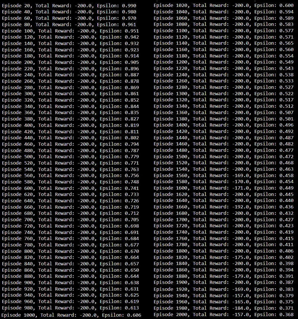
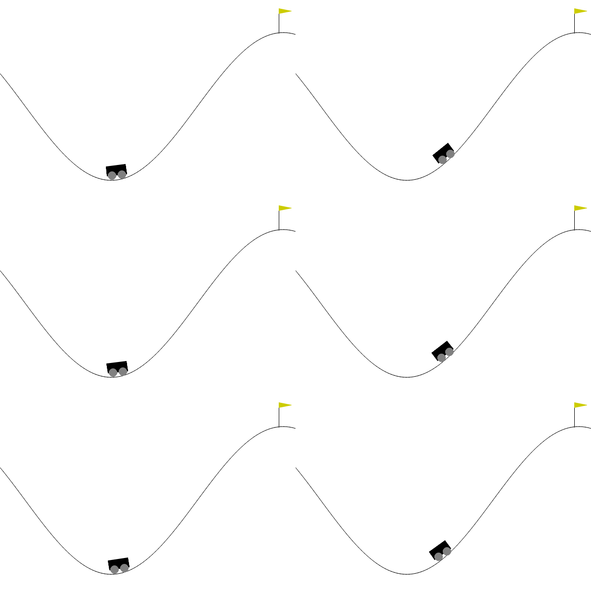
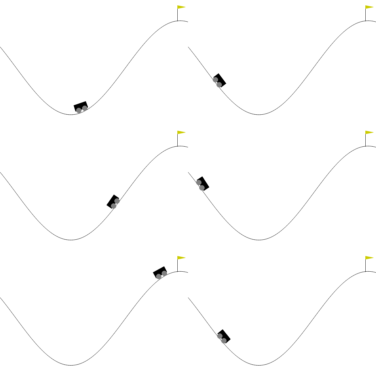
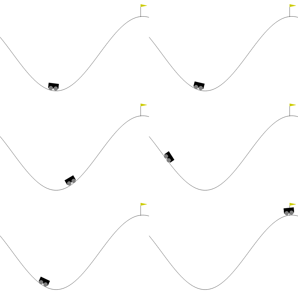
Here’s how our agent looked at different checkpoints:
- Episode 1
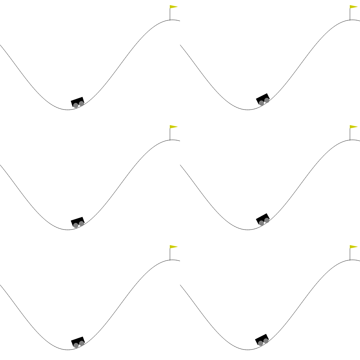
- Episode 500
- Episode 1500
- Episode 2000
Plotting Rewards Over Episodes:
plt.figure(figsize=(20, 10))
plt.plot(reward_history)
plt.xlabel('Episode')
plt.ylabel('Total Reward')
plt.title('DQN on MountainCar')
plt.show()
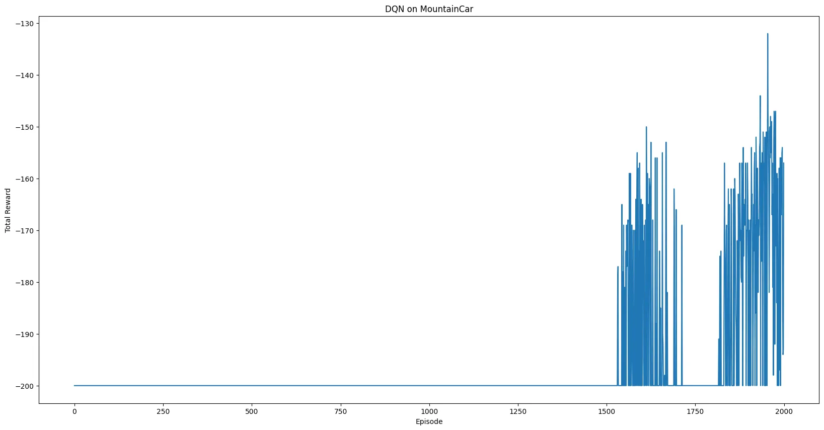
I used Matplotlib library to plot the agent’s performance, turning the list of rewards from each episode into a line graph which shows its learning progress over time:
Personal Takeaways
Honestly, watching the output was a real rollercoaster. After reading the theory, I had this idea in my head that once the agent got its first successful reward (episode 1560), the graph would shoot up in a nice clean line.
But Reinforcement Learning isn’t simple like that.
As you can see from my output and graph, my agent had its first breakthrough at 1560, but then its performance went up and down like crazy. It had a great run of -169, then dumbed down and failed after 2 more steps. My agent got stuck because its epsilon (exploration rate) dropped so low, it didn’t have enough confidence to find a better solution. So, the success of our agent depends mostly on how we set up the rules and learning process.
But even with this instability, the upward trend is very clear. So, it did learn, and was able to reach the target quite a few times, towards the end (which felt like a huge win to me!)
Note: The time limit I set was -200. So as long as the reward is greater than that, it means my agent reached the target.
Conclusion
My journey into RL began with a simple question “How do these self-driving cars that are so hyped rn even work?”, so I began to explore RL, and I was hooked in this trial-and-error process because it just felt so ‘human’.
So, why isn’t RL talked about as much as other fields amongst beginners? I think it’s because it can come off as intimidating. It doesn’t start with a nice, organized dataset, so you often have to build a whole interactive environment for the agent to learn in. And as my results show, this training is really unstable and requires a lot of patience and tweaking.
That’s exactly why I wanted to write this blog. To document my own journey from literal zero knowledge to a working (if a lil clumsy) agent and show that it’s a really rewarding challenge to take on!
I hope curious learners like me found this blog helpful and feel inspired to start their own exploration.
✍️ Written By

Devanshi Kashyap
Author • Researcher • Learner